PyTorch in Practice: Essential Building Blocks for Modern Deep Learning

From Tensors to Neural Networks: Understanding Core Components

Introduction

As deep learning continues to advance artificial intelligence applications, PyTorch has established itself as a fundamental framework powering everything from computer vision systems to large language models. Originally developed by Meta’s AI Research lab, PyTorch combines Python's flexibility with deep learning capabilities through a powerful, intuitive interface.

Photo by Iker Urteaga on Unsplash

Core Components of PyTorch

PyTorch's architecture rests on three key components that work together to enable efficient deep learning development:

1. Dynamic Tensor Library

   • Extends NumPy's array programming capabilities

   • Provides seamless CPU and GPU acceleration

   • Implements efficient mathematical operations for deep learning computations

2. Automatic Differentiation Engine (Autograd)

   • Computes gradients automatically through computational graphs

   • Manages backpropagation for neural network training

3. Deep Learning Framework

   • Delivers modular neural network components

   • Implements optimized loss functions and optimizers

Getting Started with PyTorch

Installation and Setup

PyTorch can be installed directly using pip, Python's package installer:

pip install torch

However, for optimal performance, it's recommended to install the version specifically compatible with your system's hardware. Visit pytorch.org to get the appropriate installation command based on your:

• Operating system

• Package manager preference (pip/conda)

• CUDA version (for GPU support)

• Python version

GPU Support and Compatibility

PyTorch seamlessly integrates with NVIDIA GPUs through CUDA. To verify GPU availability in your environment:

import torch

# Check GPU availability
gpu_available = torch.cuda.is_available()
print(f"GPU Available: {gpu_available}")

# Get GPU device count if available
if gpu_available:
    print(f"Number of GPUs: {torch.cuda.device_count()}")

If a GPU is detected, you can move tensors and models to GPU memory using:

# Create a tensor
tensor = torch.tensor([1.0, 2.0, 3.0])

# Move to GPU if available
device = "cuda" if torch.cuda.is_available() else "cpu"
tensor = tensor.to(device)

Apple Silicon Support

For users with Apple M1/M2/M3 chips, PyTorch provides acceleration through the Metal Performance Shaders (MPS) backend. Verify MPS availability:

import torch

# Check MPS (Metal Performance Shaders) availability
mps_available = torch.backends.mps.is_available()
print(f"MPS Available: {mps_available}")

# If MPS is available, you can use it as device
if mps_available:
    device = torch.device("mps")
    # Move tensors/models to MPS device
    tensor = tensor.to(device)

For ease of usage, I recommend using Google Colab i.e. a popular jupyter notebook–like environment, which provides time-limited access to GPUs.

Understanding Tensors

What Are Tensors?

Tensors are mathematical objects that generalize vectors and matrices to higher dimensions. In PyTorch, tensors serve as fundamental data containers that hold and process multi-dimensional arrays of numerical values. These containers enable efficient computation and automatic differentiation, making them essential for deep learning operations. PyTorch tensors are similar to Numpy arrays in basic sense.

Scalers, Vectors, Matrices and Tensors

Source: https://dev.to/mmithrakumar/scalars-vectors-matrices-and-tensors-with-tensorflow-2-0-1f66

As mentioned earlier, PyTorch tensors are data containers for array-like structures. A scalar is a zero-dimensional tensor (for instance, just a number), a vector is a one-dimensional tensor, and a matrix is a two-dimensional tensor. There is no specific term for higher-dimensional tensors, so we typically refer to a three-dimensional tensor as just a 3D tensor, and so forth. We can create objects of PyTorch’s `Tensor` class using the `torch.tensor` function as shown in the following listing.

import torch

# Scalar (0-dimensional tensor)
scalar = torch.tensor(1)     

# Vector (1-dimensional tensor)
vector = torch.tensor([1, 2, 3])    

# Matrix (2-dimensional tensor)
matrix = torch.tensor([[1, 2], 
                      [3, 4]])     

# 3-dimensional tensor
tensor3d = torch.tensor([[[1, 2], [3, 4]], 
                        [[5, 6], [7, 8]]])

Each tensor type maintains its specific dimensionality, accessible through the .shape attribute:

print(f"Scalar shape: {scalar.shape}")      # torch.Size([])
print(f"Vector shape: {vector.shape}")      # torch.Size([3])
print(f"Matrix shape: {matrix.shape}")      # torch.Size([2, 2])
print(f"3D tensor shape: {tensor3d.shape}") # torch.Size([2, 2, 2])

Tensor Data Types and Precision

PyTorch supports various data types with different precision levels, optimized for different computational needs:

Some of the common torch datatypes available with torch are float32, float64, float16, bfloat16, int8, uint8, int16, int32, int64.

The choice of precision impacts both memory usage and computational efficiency:

• float32: Standard for most deep learning tasks

• float16: Reduced precision, useful for memory optimization

• bfloat16: Brain Floating Point, balances precision and range

Floating Data Types

PyTorch supports various floating-point precisions for tensors, each serving different computational needs:

• torch.float32 (default): 32-bit precision offering 6-9 decimal places, optimal for most deep learning tasks

• torch.float64: 64-bit double precision with 15-17 decimal places, suitable for high-precision numerical computations

• torch.float16: 16-bit half precision with 3-4 decimal places, useful for memory-efficient operations

• torch.bfloat16: Brain floating point format with 2-3 decimal precision, balancing range and precision

import torch

float32_tensor = torch.tensor([1.0, 2.0], dtype=torch.float32)  
float64_tensor = torch.tensor([1.0, 2.0], dtype=torch.float64)  
float16_tensor = torch.tensor([1.0, 2.0], dtype=torch.float16)  
bfloat16_tensor = torch.tensor([1.0, 2.0], dtype=torch.bfloat16)

Integer Types

PyTorch supports various integer data types, each with specific memory allocations and value ranges:

• int8: 8-bit signed integers (-128 to 127)

• uint8: 8-bit unsigned integers (0 to 255)

• int16: 16-bit signed integers (-32768 to 32767)

• int32: 32-bit signed integers (-2^31 to 2^31-1)

• int64: 64-bit signed integers (-2^63 to 2^63-1), default integer type in PyTorch

import torch

int8_tensor = torch.tensor([1, 2], dtype=torch.int8)     
uint8_tensor = torch.tensor([1, 2], dtype=torch.uint8)   
int16_tensor = torch.tensor([1, 2], dtype=torch.int16)   
int32_tensor = torch.tensor([1, 2], dtype=torch.int32)   
int64_tensor = torch.tensor([1, 2], dtype=torch.int64)

Datatype Conversion

We can convert tensors from one datatype to another using the .to method.

# Converting between data types
tensor = torch.tensor([1, 2, 3])
float_tensor = tensor.to(torch.float32) # Convert from int64 to float32
int_tensor = tensor.to(torch.int32)     # Convert from float32 to int32

Common Tensor Operations

PyTorch provides several fundamental tensor operations essential for deep learning computations. Here are the key operations with their implementations and specific use cases.

1. Tensor Creation and Shape Manipulation

Creating tensors and understanding their shape are fundamental operations in PyTorch:

import torch

# Create 2D tensor
tensor2d = torch.tensor([[1, 2, 3], 
                        [4, 5, 6]])

# Check tensor shape
shape = tensor2d.shape  
# Returns: torch.Size([2, 3])

For the above tensor, the shape if 2 x 3 i.e. 2 rows and 3 columns. We can change the shape of the array by maintaining the total size of the array using reshape method.

2. Reshaping Operations

PyTorch offers two methods for tensor reshaping:

# Reshape tensor from (2,3) to (3,2)
reshaped_tensor = tensor2d.reshape(3, 2)

# Alternative using view
viewed_tensor = tensor2d.view(3, 2)

Technical Note: .view() and .reshape() differ in memory handling:

• .view(): Requires contiguous memory layout

• .reshape(): Works with any memory layout, performs copy if necessary

3. Matrix Operations

PyTorch implements efficient matrix operations essential for linear algebra computations:

# Transpose operation
transposed = tensor2d.T

# Matrix multiplication methods
result1 = tensor2d.matmul(tensor2d.T)  # Using matmul
result2 = tensor2d @ tensor2d.T        # Using @ operator

Output shapes for a 2x3 input tensor:

• Transpose: 3x2

• Matrix multiplication with transpose: 2x2

These operations form the foundation for neural network computations and linear algebra operations in deep learning models. For an exhaustive list of tensor operations, refer to the PyTorch documentation.

Automatic Differentiation

Understanding Computational Graphs

PyTorch builds computational graphs that track operations performed on tensors. These graphs enable automatic differentiation through the autograd system, making gradient computation efficient and programmatic.

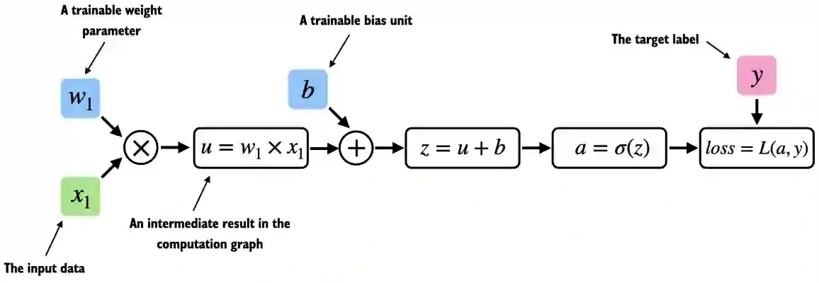
A computational graph is a directed graph that allows us to express and visualize mathematical expressions. In the context of deep learning, a computation graph lays out the sequence of calculations needed to compute the output of a neural network—we will need this to compute the required gradients for backpropagation, the main training algorithm for neural networks.

Consider the following example of a single layer neural network performing logistic regression with single weight and bias.

import torch
import torch.nn.functional as F

# Initialize inputs and parameters
y = torch.tensor([1.0])           # Target
x1 = torch.tensor([1.1])          # Input
w1 = torch.tensor([2.2], 
                  requires_grad=True)  # Weight
b = torch.tensor([0.0], 
                 requires_grad=True)   # Bias

# Forward pass computation
z = x1 * w1 + b                   # Linear computation
a = torch.sigmoid(z)              # Activation
loss = F.binary_cross_entropy(a, y)    # Loss computation

We have used the torch.nn.functional module from torch which provides many utility functions like loss functions, activations etc required to write and train deep neural networks.

Source: LLMs from Scratch

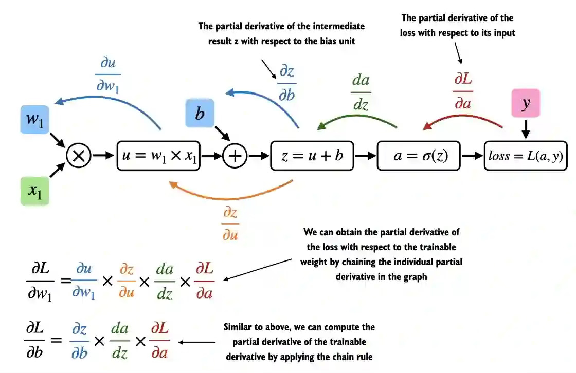
Gradient Computation with Autograd

To train the above model, we have to compute the gradients of loss w.r.t w1 and b which will be further used to update the existing weights iteratively. This is where PyTorch makes our life easier by automatically calculating them using the autograd engine.

Source: LLMs from Scratch

PyTorch's autograd system automatically computes gradients for all tensors with requires_grad=True. Here's how to compute gradients:

from torch.autograd import grad

# Manual gradient computation
grad_L_w1 = grad(loss, w1, retain_graph=True)
grad_L_b = grad(loss, b, retain_graph=True)

# Alternative using backward()
loss.backward()
print(w1.grad)    # Access gradient for w1
print(b.grad)     # Access gradient for b

Technical Note: When using backward():

• Gradients accumulate by default

• Use zero_grad() before each backward pass in training loops

• retain_graph=True allows multiple backward passes

The grad function is used to get gradients manually and it is useful for debugging and demonstration purposes. Using the backward() function automatically calculates for all the tensors which has requires_grad=True set and gradients will be stored inside .grad property.

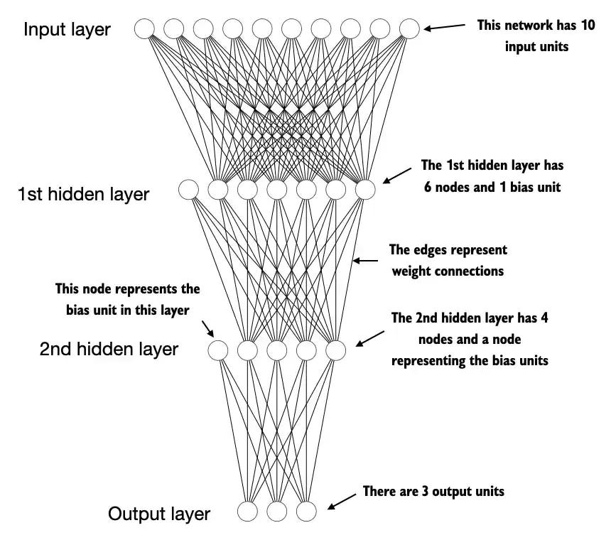
Building Neural Networks with PyTorch

Next, we focus on PyTorch as a library for implementing deep neural networks. While our previous example demonstrated a single neuron for classification, practical applications require complex architectures like transformers and ResNets that process multiple inputs through various hidden layers to produce outputs. Manually calculating and updating individual weights becomes impractical at this scale. PyTorch provides a structured approach through its neural network modules, enabling efficient implementation of sophisticated architectures.

Source: LLMs from Scratch

Introduction to torch.nn.Module

The torch.nn.Module serves as PyTorch's foundational class for neural networks, providing a systematic way to define and manage model architectures, parameters, and computations. This base class handles essential functionalities including parameter management, device placement, and training behaviors.

The subclass has the following components:

• __init__: We define the layers of neural networks in the constructor of the subclass defined and how the layers interact during forward propagation.

• forward: The forward method describes how the input data passes through the network and comes together as a computation graph.

Creating Custom Neural Network Architectures

Complex neural networks require multiple layers with specific activation functions. Here's a practical implementation of a multi-layer neural network:

class DeepNetwork(nn.Module):
    def __init__(self, num_inputs, num_outputs):
        super().__init__()
        
        self.layers = nn.Sequential(
            nn.Linear(num_inputs, 30),     # First hidden layer
            nn.ReLU(),                     # Activation function
            nn.Linear(30, 20),             # Second hidden layer
            nn.ReLU(),                     
            nn.Linear(20, num_outputs)      # Output layer
        )

    def forward(self, x):
        return self.layers(x)

nn.Sequential provides a container for stacking layers in a specific order, streamlining the forward pass implementation.

Model Parameters and Initialization

PyTorch automatically handles parameter initialization, but you can access and modify parameters:

model = DeepNetwork(50, 3)

# Count trainable parameters
num_params = sum(p.numel() for p in model.parameters() if p.requires_grad)
print(f"Trainable parameters: {num_params}")

# Access layer parameters
for name, param in model.named_parameters():
    print(f"Layer: {name} | Size: {param.size()}")

# Custom initialization
def init_weights(m):
    if isinstance(m, nn.Linear):
        torch.nn.init.xavier_uniform_(m.weight)
        m.bias.data.fill_(0.01)

model.apply(init_weights)

Each parameter for which requires_grad=True counts as a trainable parameter and will be updated during training. In the above code, this referes to the weights initialized in torch.nn.Linear layers.

Forward Propagation Implementation

Forward propagation defines how input data flows through the network. Let's initialise random values and pass it through the model.

# Sample forward pass
model = DeepNetwork(50, 3)
batch_size = 32
input_features = torch.randn(batch_size, 50)

with torch.no_grad():
    outputs = model(input_features)

print(f"Output shape: {outputs.shape}")

Training Mode vs. Evaluation Mode

PyTorch models have distinct training and evaluation modes that affect certain layers' behavior:

model = DeepNetwork(50, 3)

# Training mode
model.train()
training_output = model(input_features)  # Layers like Dropout and BatchNorm active

print(training_output)

# Evaluation mode
model.eval()
with torch.no_grad():
    eval_output = model(input_features)  # Deterministic behavior
    print(eval_output)

PyTorch models operate in two distinct modes:

1. Training Mode (model.train()):

   • Activates Dropout and BatchNorm layers

   • Enables gradient computation and tracking

   • Maintains computational graph for backpropagation

2. Evaluation Mode (model.eval() with torch.no_grad()):

   • Disables Dropout and freezes BatchNorm statistics

   • Prevents gradient computation and tracking

   • Optimizes memory usage by eliminating gradient storage

   • Reduces computational overhead during inference

This mode management ensures efficient resource utilization while maintaining appropriate model behavior for both training and inference phases.

Efficient Data Handling

Efficient data handling is crucial for developing robust deep learning models. PyTorch provides two primary tools for data management: the Dataset and DataLoader classes.

1. Dataset and DataLoader Overview

PyTorch's data handling framework consists of

• Dataset: Defines data access and preprocessing

• DataLoader: Handles batch creation, shuffling, and parallel loading

Let's implement a simple classification dataset to demonstrate these concepts:

import torch
from torch.utils.data import Dataset, DataLoader

# Training classification data
X_train = torch.tensor([
    [-1.2, 3.1],
    [-0.9, 2.9],
    [-0.5, 2.6],
    [2.3, -1.1],
    [2.7, -1.5]
])
y_train = torch.tensor([0, 0, 0, 1, 1])

# Testing dataset
X_test = torch.tensor([
    [-0.8, 2.8],
    [2.6, -1.6],
])
y_test = torch.tensor([0, 1])

2. Creating Custom Dataset Objects

Next, we create a custom dataset class, SampleDataset, by subclassing from PyTorch’s Dataset parent class. It has following properties:

• __init__: Initialize dataset attributes.

• __getitem__: Define data access for individual samples

• __len__: Return total number of samples

from torch.utils.data import Dataset

class SampleDataset(Dataset):
    def __init__(self, X, y):
    """Initialize the dataset with features and labels"""
        self.features = X
        self.labels = y

    def __getitem__(self, index):
    """Retrieve a single example and its label"""     
        one_x = self.features[index]     
        one_y = self.labels[index]       
        return one_x, one_y              

    def __len__(self):
    """Get the total number of examples in the dataset"""
        return self.labels.shape[0]     

train_ds = SampleDataset(X_train, y_train)
test_ds = SampleDataset(X_test, y_test)

3. Implementing DataLoader

DataLoaders handle the heavy lifting of batching, shuffling, and parallel data loading. Now we can create DataLoaders from the SampleDataset object created. This can be done as follows:

# Create DataLoader with specific configurations
train_loader = DataLoader(
    dataset=train_ds,     # Dataset Instance
    batch_size=2,         # Number of samples per batch
    shuffle=True,         # Shuffle the training data
    num_workers=0         # Number of parallel workers
    drop_last=True.       # Drop incomplete batch
)

test_loader = DataLoader(
    dataset=test_ds,
    batch_size=2,
    shuffle=False,        # No need to shuffle test data
    num_workers=0
)

Some key parameters of Dataloaders class are as follows:

• dataset: The Dataset instance to load data from

• batch_size: Number of samples per batch

• shuffle: Whether to shuffle data between epochs

• num_workers: Number of subprocesses for data loading

• drop_last: Whether to drop the last incomplete batch

• pin_memory: Pin memory for faster data transfer to GPU

Complete Example with Best Practices (Best Practice)

Here's a comprehensive implementation incorporating all concepts:

import torch
from torch.utils.data import Dataset, DataLoader

class SampleDataset(Dataset):
    def __init__(self, X, y, transform=None):
        self.features = X
        self.labels = y
        self.transform = transform # Input transformations if required
    
    def __getitem__(self, index):
        x = self.features[index]
        y = self.labels[index]
        
        if self.transform:
            x = self.transform(x)
            
        return x, y
    
    def __len__(self):
        return len(self.labels)

# Configuration for optimal performance
def create_data_loader(dataset, batch_size, is_training=True):
    return DataLoader(
        dataset=dataset,
        batch_size=batch_size,
        shuffle=is_training,
        num_workers=4 if is_training else 2,
        pin_memory=torch.cuda.is_available(),
        drop_last=is_training,
        persistent_workers=True
    )

# Usage example
if __name__ == "__main__":
    # Create dataset
    dataset = SampleDataset(X_train, y_train)
    
    # Create data loader
    train_loader = create_data_loader(
        dataset=dataset,
        batch_size=32,
        is_training=True
    )
    
    # Training loop example
    for epoch in range(num_epochs):
        for batch_idx, (features, labels) in enumerate(train_loader):
            # Training operations here
            pass

This implementation provides a robust foundation for handling data in PyTorch, incorporating best practices for memory management and parallel processing. Adjust the configurations based on your specific use case and available computational resources.

Implementing Training Loops in PyTorch

A PyTorch training loop consists of several key components:

• model initialization,

• optimizer configuration,

• loss function definition, and

• the iterative training process.

Here's a structured implementation showcasing these elements.

Basic Training Loop Structure (Best Practice)

import torch
import torch.nn as nn
from torch.optim import Adam
from torch.utils.data import DataLoader

def train_model(
    model: nn.Module,
    train_loader: DataLoader,
    val_loader: DataLoader,
    num_epochs: int,
    learning_rate: float,
    device: str = 'cuda' if torch.cuda.is_available() else 'cpu'
) -> dict:
    
    # Initialize optimizer and loss function
    optimizer = Adam(model.parameters(), lr=learning_rate)
    criterion = nn.CrossEntropyLoss()
    
    # Move model to device
    model = model.to(device)
    
    # Training history
    history = {
        'train_loss': [],
        'val_loss': [],
        'val_accuracy': []
    }
    
    # Training loop
    for epoch in range(num_epochs):
        # Training phase
        model.train()
        train_loss = 0.0
        
        for batch_idx, (features, labels) in enumerate(train_loader):
            # Move data to device
            features = features.to(device)
            labels = labels.to(device)
            
            # Forward pass
            outputs = model(features)
            loss = criterion(outputs, labels)
            
            # Backward pass and optimization
            optimizer.zero_grad()
            loss.backward()
            optimizer.step()
            
            # Accumulate loss
            train_loss += loss.item()
            
            # Optional: Print batch progress
            if batch_idx % 100 == 0:
                print(f'Epoch: {epoch+1}/{num_epochs} | '
                      f'Batch: {batch_idx}/{len(train_loader)} | '
                      f'Loss: {loss.item():.4f}')
        
        # Calculate average training loss
        train_loss = train_loss / len(train_loader)
        history['train_loss'].append(train_loss)
        
        # Validation phase
        model.eval()
        val_loss = 0.0
        correct = 0
        total = 0
        
        with torch.no_grad():
            for features, labels in val_loader:
                features = features.to(device)
                labels = labels.to(device)
                
                # Forward pass
                outputs = model(features)
                loss = criterion(outputs, labels)
                
                # Accumulate validation metrics
                val_loss += loss.item()
                _, predicted = torch.max(outputs.data, 1)
                total += labels.size(0)
                correct += (predicted == labels).sum().item()
        
        # Calculate validation metrics
        val_loss = val_loss / len(val_loader)
        val_accuracy = 100 * correct / total
        
        # Store validation metrics
        history['val_loss'].append(val_loss)
        history['val_accuracy'].append(val_accuracy)
        
        # Print epoch summary
        print(f'Epoch: {epoch+1}/{num_epochs} | '
              f'Train Loss: {train_loss:.4f} | '
              f'Val Loss: {val_loss:.4f} | '
              f'Val Accuracy: {val_accuracy:.2f}%')
    
    return history

# Example Usage
def main():
    # Assume we have model and data loaders defined
    model = DeepNetwork()
    
    # Training configuration
    config = {
        'num_epochs': 10,
        'learning_rate': 0.001,
    }
    
    # Train model
    history = train_model(
        model=model,
        train_loader=train_loader,
        val_loader=test_loader,
        num_epochs=config['num_epochs'],
        learning_rate=config['learning_rate']
    )

The training loop does the following gradient descent as following:

• The training process involves passing logits to the cross_entropy loss function, which internally applies softmax for optimized performance and numerical stability.

• The loss.backward() call computes gradients through PyTorch's computational graph

• The optimizer.step() step updates the model parameters using these gradients

• The optimizer.zero_grad() must be called every training iteration to reset gradients, preventing unintended accumulation that could distort the optimization process.

Model Persistence in PyTorch: Saving and Loading

PyTorch provides efficient mechanisms for model persistence through its state dictionary system. The state dictionary (state_dict) maintains a mapping between layer identifiers and their corresponding parameters (weights and biases).

Basic Model Persistence

Saving Models

After training the model, it is necessary to save the model weights to reuse later for further training or deployment. Save a model's learned parameters using the state dictionary:

import torch

# Save model parameters
torch.save(model.state_dict(), "model_parameters.pth")

Loading Models

The torch.load("model_parameters.pth") function reads the file "model_parameters.pth" and reconstructs the Python dictionary object containing the model’s parameters while model.load_state_dict() applies these parameters to the model, effectively restoring its learned state from when we saved it.

We need the instance of the model in memory to apply the saved parameters. Here, the NeuralNetwork(2, 2) architecture needs to match the original saved model exactly.

# Initialize model architecture
model = NeuralNetwork(num_inputs=2, num_outputs=2)

# Load saved parameters
model.load_state_dict(torch.load("model_parameters.pth"))

Comprehensive Model Persistence (Best Practice)

For production scenarios, save additional information alongside model parameters:

# Save complete model state
checkpoint = {
    'model_state_dict': model.state_dict(),
    'optimizer_state_dict': optimizer.state_dict(),
    'epoch': epoch,
    'loss': loss,
    'model_config': {
        'num_inputs': 2,
        'num_outputs': 2
    }
}
torch.save(checkpoint, "model_checkpoint.pth")

# Load complete model state
checkpoint = torch.load("model_checkpoint.pth")
model = NeuralNetwork(**checkpoint['model_config'])
model.load_state_dict(checkpoint['model_state_dict'])
optimizer.load_state_dict(checkpoint['optimizer_state_dict'])
epoch = checkpoint['epoch']
loss = checkpoint['loss']

Conclusion

PyTorch's architecture provides a robust foundation for deep learning development through its integrated components: tensor computations, automatic differentiation, and neural network modules. The framework's design enables efficient model implementation through dynamic computation graphs, GPU acceleration, and intuitive APIs for data processing and model construction.

For continued learning and implementation guidance, refer to PyTorch's official documentation which provides comprehensive updates on best practices, optimizations, and emerging capabilities. This ensures your deep learning applications remain aligned with current framework standards and performance benchmarks.

---

Thanks for reading NeuraForge: AI Unleashed!

If you enjoyed this deep dive into AI/ML concepts, please consider subscribing to our newsletter for more technical content and practical insights. Your support helps grow our community and keeps the learning going! Don't forget to share with peers who might find it valuable. 🧠✨