Value-Based Policy Training in Reinforcement Learning

Insights in a Jiffy #5: How Agents Use State-Value and Action-Value Functions to Optimize Choices

Introduction

Reinforcement Learning (RL) is a branch of artificial intelligence that focuses on creating agents capable of making smart decisions by interacting with their environment through trial and error. This interaction is facilitated by a feedback loop involving states, actions, and rewards. The environment provides a state, the agent takes an action, and the environment responds with a reward and a new state. The goal of RL is to find a policy that maximizes the expected return when the agent acts according to it.

Photo by Owen Beard on Unsplash

Policy and Decisions - Recap

At the heart of RL is the concept of a policy, which determines what action to take given the current state. Policies can be deterministic, always returning the same action for a given state, or stochastic, outputting a probability distribution over possible actions. The ultimate goal is to find the optimal policy (π*) that maximizes the expected return.

There are two approaches to finding an optimal policy for the RL problem at hand:

Policy-based Approach

• Policy-based methods directly train the policy to determine which action to take in a given state.

• This is achieved by optimizing the policy function to maximize the expected rewards. The policy is typically represented by a neural network and is trained without a value function (used to tell how good the agent is at particular state or to take particular action - Used in Value based Approach).

• The policy is not defined by hand but is learned through training.

Value-Based Approach

• Value-based methods work indirectly by learning a value function that estimates how good it is to be in a particular state or which action to take in a given state.

• The value function is trained in value based approach and the policy is defined by hand i.e. there is a fixed policy function. For example, a greedy policy always chooses the action/state that leads to the highest value.

• Based on the information provided by the Value function (i.e. usually which state is more valuable or which action is best to take), the policy will decide the next action/state to move to.

In value-based methods, the link between the value function and policy is crucial. The policy uses the value function to make decisions. The trained value function outputs the action-value pair for each state, which is used by the predefined policy function to choose the relevant action.

For example, the epsilon-greedy policy balances exploration and exploitation by choosing the action with the highest value most of the time but occasionally selects a random action.

Going on we will focus more on the Value based functions and its different variations.

Different types of Value based Functions

There are two types of value based functions that can be used to to get the expected return or reward for agent to take a decision according to a fixed policy.

State-Value Function

The state-value function, V(s), outputs the expected return if the agent starts in a state s and follows the policy forever afterward. It is defined as:

\(V(s) = \mathbb{E} \left[ R_t + \gamma R_{t+1} + \gamma^2 R_{t+2} + \cdots \mid S_t = s \right] \)

Interpretation:

• Rt: The immediate reward received at time t.

• γ: The discount factor, which determines how much future rewards are valued compared to immediate rewards.

• S_t = s: The condition that the agent is in state s at time t.

This formula calculates the expected cumulative reward starting from state s and following the policy. It considers the immediate reward and the discounted future rewards.

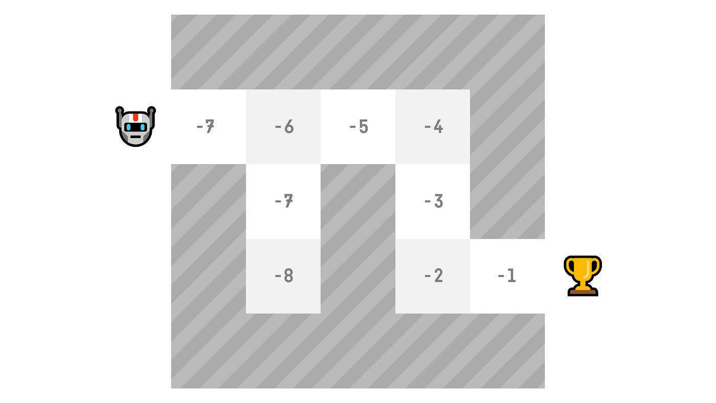
Imagine a maze where each state has a value representing how good it is to be in that state. The state-value function assigns these values based on the expected return from starting in that state and following the policy.

Source: https://thomassimonini.medium.com/an-introduction-to-deep-reinforcement-learning-17a565999c0c

Action-Value Function

The action-value function, Q(s,a), returns the expected return if the agent starts in state s, takes action a, and then follows the policy forever after. It is defined as:

\(Q(s,a) = \mathbb{E} \left[ R_t + \gamma R_{t+1} + \gamma^2 R_{t+2} + \cdots \mid S_t = s, A_t = a \right]\)

Interpretation:

• Rt: The immediate reward received at time t.

• γ: The discount factor, which determines how much future rewards are valued compared to immediate rewards.

• S_t = s: The condition that the agent is in state s at time t.

• A_t = a: The condition that the agent takes action a at time t.

Visual Representation:
Picture a similar maze but with each state-action pair having a value. The action-value function evaluates how good it is to take a specific action in a given state, considering the expected return from that action and the subsequent policy.

The need for Bellman Equation

In the different types of Value Functions mentioned above, we can see that the expected return to make a decision/take an action depends on agent starting in a state s and following the policy forever or until the episode ends and then summing the rewards. This is a computationally expensive process if it has to be repeated at every state.

The Bellman equation provides a solution by breaking down the value function into smaller, manageable parts. It simplifies the calculation by considering the immediate reward and the discounted value of the next state:

\(V(s) = \max_a \left( R(s,a) + \gamma V(s') \right) \)

Interpretation:

• V(s): The value of being in state s.

• R(s,a): The immediate reward received when taking action a in state s.

• γ: The discount factor, which determines how much future rewards are valued compared to immediate rewards.

• V(s'): The value of the next state s'.

This recursive equation allows for efficient computation of state values without needing to calculate the expected return for each state from scratch. The Bellman equation is crucial for making value-based methods computationally feasible.

Conclusion

Understanding these concepts is essential for grasping the fundamentals of reinforcement learning. The Bellman equation plays a pivotal role in making value-based methods efficient, and visualizing state-value and action-value functions helps in understanding how agents make decisions based on these values.

---

This article is part of our ongoing series on Reinforcement Learning and represents Issue #5 in the "Insights in a Jiffy" collection. We encourage you to read our previous issues in this series for a more comprehensive understanding here. Each article builds upon the concepts introduced in earlier posts, providing a holistic view of the Reinforcement Learning landscape.

If you enjoyed this blog, please click the ❤️ button, share it with your peers, and subscribe for more content. Your support helps spread the knowledge and grow our community.